Production Function: How to Calculate with Formula & Example
What is the Production Function?
The production function is the calculation by which the number of inputs creates a number of outputs. In other words, it states the relationship between inputs and outputs. So how much would x number of inputs be able to produce. For example, a firm may have 5 workers producing 100 pins an hour. If the firm hires another 5 employees alongside 100 pin supplies, then the production function would suggest 100 pins would be produced.
There are four main factors of production – land, labour, capital, and entrepreneurship. With regards to the production function, these factors would usually be included in the inputs which create x number of outputs. The number of which will depend on the production function which will vary from product to product.
Key Points
- The production function is a mathematical equation that calculates the maximum output a firm can achieve with a selected number of inputs (capital, labour, and land).
- The production function can be calculated using the formula: Q = f(Capital, Land, Labour), where the inputs are a function of the output.
- The production function comes in two phases – the short-run and the long-run.
Some key concepts and measurements include:
Total Product: the total product of a firm refers to the number of goods that it produces. In other words, it is simply the total output.
Average Product: the average product measures the output per worker or output per unit of capital.
Marginal Product: the marginal product refers to the additional output achieved by employing an additional unit of input. For instance, an additional worker may be able to produce an extra 5 units. This is referred to in the short-run.
Production Function Formula
The production function can be seen using the formula for its inputs. This looks something like: Q = f (Input#1, Input#2, Input#3, Input#4….). This would represent the four factors of production in land, labour, capital, and entrepreneurship. So the quantity output is dependant on the various inputs from land, labour, capital, and entrepreneurship. Let us now look at an example.
Production Function Example & How to Calculate
Bob’s Burgers is a business that sells hamburgers to consumers. It has three main inputs – burger ingredients (land/natural resources), cooker (capital), and an employee (labor). These variables come together to form the production function which stipulates how much output will be achieved from a specific number of inputs.
In this example, there are ingredients that are needed in the form of buns and hamburgers, which is input number one. There is also a cooker which is needed which can cook 6 hamburgers every half hour. However, those cannot be cooked on their own, so an employee is needed. They can produce 5 burgers every ten minutes. The production function can therefore be constructed as per below:

This formula calculates how the output achieved when all variables are considered as part of the production function. One important point to note is that the output is naturally limited to the minimum number of outputs any variable can produce. For instance, if there is only enough ingredients for one burger, then only one burger is made. If there is only one cooker, then only 12 burgers can be made. Similarly, if there is only one employee, then only 30 burgers can be made.
Production Function Short-Run
The production function in the short run is where at least one input is fixed. For example, with regards to Bob’s Burgers in the previous section, its relatively easy to get ingredients, so this is not a fixed input. However, it takes one month to increase the number of cookers, so there is a one month lead time to increase production.
Similarly, there is a two week lead time to hire an additional employee. So when it comes to the short-run in the production function, this occurs at the maximum point by which it would take to increase production. In this example, that would occur in the one month it takes to bring in an additional cooker. Until this new cooker is received, output per hour cannot increase as production is naturally limited by this input.
There are two main points to understand about the production function in the short-run:
- The production function in the short-run occurs when one of the inputs is fixed. Most frequently, this is capital.
- A business has set its production to this short-term rate.
In the short-run, the business cannot expand production as it needs additional input to do so. The time it takes to acquire this input is known as the short-run and it can vary depending on the good being produced.
Diminishing Marginal Returns
In the short-run, the law of diminishing returns states that as production increases within the production function, diminishing returns can occur. To explain, marginal product is an important concept to understand. It refers to the additional output achieved from an additional unit of input. For example, one additional worker producers one additional unit, which is the marginal product.
If we take an example of a bakery. When there are 0 bakers present, then 0 loaves of bread are produced. When one baker is employed, they are able to make 2 loaves of bread. This is known as the marginal product and can be calculated by using the formula: change in quantity / change in workers. For example, when an additional baker is hired at 2 bakers, the output increases to 5 loaves of bread. So quantity increases by 3 as the number of workers increases by 1, which would equal 3/1 = 3 as the marginal product.
| # Bakers | 1 | 2 | 3 | 4 | 5 |
| # Bread (TP) | 2 | 5 | 7 | 8 | 8 |
| Marginal Product (MP) | 2 | 3 | 2 | 1 | 0 |
In this example, the concept of diminishing marginal returns kicks in at 3 bakers as the marginal product starts to decrease. This is because production starts to become less efficient. Perhaps workers start getting in each others way, they are chatting with each other more, or perhaps there is a limited usage of the oven.
Let us take another example. There is a cafe that has three coffee machines that can produce 40 cups of coffee per hour. It also has three employees that can make 30 cups of coffee per hour. In total, the coffee machines can produce 120 cups of coffee per hour when they are being fully utilised. At 3 employees, the cafe can produce 90 cups of coffee – well below the capacity of their machines. So they hire an additional worker.
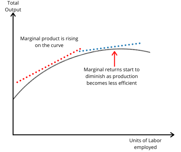
The problem, however, is that there are only 3 machines between 4 workers. In turn, the productivity of the employees decreases as they start to get in each other’s way. So even though output may increase, the marginal increase is no longer 30 cups of coffee, but 15. This can be illustrated in the graph below. As more units of labor are introduced, the marginal product increases in an upward scale, presenting increasing returns to scale. However, in the short-run, the firm faces decreasing returns due to its limited capacity. In turn, the firm would need to increase its investment in the capital such as purchasing a new coffee machine.
Production Function Long-Run
In contrast to the short-run, in the long-run, every input is variable. For instance, inputs such as labor and capital can vary dramatically in the course of a year or decade. Some firms will hire thousands of additional workers, whilst others may open tens or hundreds of factories or stores. In other words, capital, labor, and land/natural resources all vary in the long run. This creates what is known as the isoquant curve.
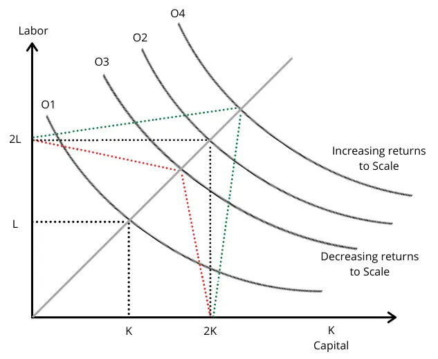
The isoquant curve explains the relationship between labor and capital, which can fluctuate depending on how much is employed. It shows potential output based on the differing level of variables input. As illustrated in the graph below, O1 demonstrates the isoquant curve where one unit of capital and one unit of labor are used.
When these variables are doubled so that two units of labor and two units of capital are used, output also doubles to point O2. However, output may not increase in line with the previous trend as it either becomes more efficient and creates increasing returns to scale, or, production becomes less efficient and creates decreasing returns to scale.
As seen at O3, there are decreasing returns to scale. This means that as production increases, the level of marginal output has started to decrease. In other words, the firm is experiencing diminishing marginal returns. Output may start to diminish for a number of reasons. For example, workers may start to get in each other’s way or duplicate each other’s work.
By contrast, the firm may benefit from increasing returns to scale as seen at O4. This is where firms benefit from economies of scale which will be looked at later in this chapter. Simply put, the efficiency of its workers increases alongside output. For instance, two workers may be able to separate tasks through the division of labor, thereby increasing the efficiency of the individual tasks and therefore creating increasing returns to scale.
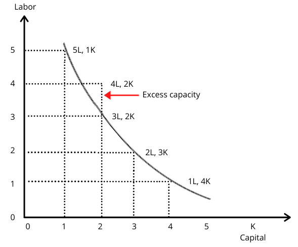
The isoquant curve can demonstrate what output levels would be at different levels of inputs. As we can see on the graph below, the isoquant curve demonstrates the maximum output at any specific level of output. For example, when there is 5 units of labor and one unit of capital, there are 5 units of output. At 3 units of labor and 2 units of capital, there are 6 units of output.
Yet at 4 units of labor and 1 unit of capital, the output does not reach the isoquant curve, which means output is below its maximum capacity at that specific amount of inputs. When 2 units of capital are introduced, the firm is able to output more units, but there is excess capacity. This may be because workers are stood idle for a period of time whilst they wait for the necessary capital equipment.
Production Function FAQs
The production function is a mathematical equation that calculates the maximum output a firm can achieve with a selected number of inputs (capital, labour, and land).
The production function can be calculated using the formula: Q = f(Capital, Land, Labour), where the inputs are a function of the output.
The production function comes in two phases – the short-run and the long-run. The short-run is simply the period by which it would take the firm to expand production beyond its maximum capacity. For instance, it may take a manufacturing firm one year to build a new factory, so anything less than this is the short-term. By contrast, the period beyond this point whereby such inputs are variable, is known as the long-term.
A production function is used to determine how changes in the inputs used in production affect the level of output produced. It can be used to identify the most efficient combination of inputs to use to produce a given level of output.
About Paul
Paul Boyce is an economics editor with over 10 years experience in the industry. Currently working as a consultant within the financial services sector, Paul is the CEO and chief editor of BoyceWire. He has written publications for FEE, the Mises Institute, and many others.

Further Reading
 White Collar: Definition & Examples - A white collar is the name used to define a segment of employees that earn higher than average wages in…
  Vertical Integration: Definition, Examples, Pros & Cons - Vertical integration is where two businesses at different stages of the supply chain join together.
  Sunk Cost: What it is, Examples & Fallacy - A sunk cost is a payment that has been made but cannot now be recovered.