Table of Contents

Indifference Curve: Definition, Formula & Examples

What is the Indifference Curve?

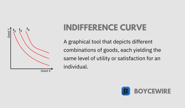
Indifference curves are a fundamental concept in microeconomics, specifically in consumer choice theory. The term “indifference curve” refers to a graphical representation of the various combinations of two goods or services that provide the same level of satisfaction or utility to a consumer.

In other words, the consumer is indifferent between any two points on the curve, as each combination provides them with the same level of happiness. This concept allows economists to analyze and understand consumer preferences and behaviors under different circumstances, such as changes in income or price levels.

Key Points

Indifference curves represent different combinations of goods that provide the same level of satisfaction or utility to an individual.
Indifference curves are downward sloping and convex to the origin, reflecting the principle of diminishing marginal rate of substitution.
The slope of an indifference curve, known as the marginal rate of substitution (MRS), indicates the rate at which an individual is willing to trade one good for another while maintaining the same level of satisfaction.

Characteristics of Indifference Curves

Indifference curves have several key properties that define their shape and position in relation to each other. These properties are essential to understanding the nature of consumer preferences and the behavior of indifference curves in various scenarios. The following are some of the fundamental properties of indifference curves:

Negatively Sloped: Indifference curves typically slope downward from left to right, indicating that as the consumption of one good increases, the consumption of the other good must decrease in order to maintain the same level of utility. This negative slope reflects the concept of trade-offs, as consumers need to give up some of one good to obtain more of the other good.
Convex to the Origin: Indifference curves are generally convex to the origin, reflecting the idea of diminishing marginal rate of substitution. As consumers consume more of one good, they are willing to give up less and less of the other good to gain additional units of the first good. This convexity implies that consumers have a preference for a diversified consumption bundle.
Higher Indifference Curves Represent Higher Utility: Indifference curves that are further from the origin represent higher levels of utility. This is because consumers would always prefer to consume more of both goods if possible, so a consumption bundle on a higher indifference curve would yield more satisfaction.
Non-Intersecting: Indifference curves cannot intersect each other. If two indifference curves were to cross, it would imply that the consumer has two different utility levels for the same consumption bundle, which contradicts the assumption that each combination of goods on an indifference curve provides the same utility.
Continuous: Indifference curves are assumed to be continuous, meaning there are no gaps or sudden jumps in the curve. This property reflects the assumption that consumer preferences are stable and consistent across different consumption bundles.

By understanding these properties, we can gain valuable insights into consumer behavior and decision-making processes, and use indifference curve analysis as a tool for predicting and explaining various economic phenomena.

Examples of Indifference Curves

Indifference curves can be used to illustrate a wide range of consumer preferences and decision-making scenarios. Here, we provide several examples to demonstrate how indifference curves can be applied in various contexts:

1. Perfect Substitutes

In cases where two goods are perfect substitutes, the indifference curves will be straight lines with a constant slope. This is because the consumer is willing to trade one good for the other at a constant rate, without any preference for diversification. For example, two brands of bottled water that have identical taste and quality would be considered perfect substitutes.

2. Perfect Complements

When two goods are perfect complements, the indifference curves take the shape of right angles. This is because the consumer derives utility only from consuming both goods in fixed proportions. An example of perfect complements could be left and right shoes: a consumer would not derive additional satisfaction from having more left shoes without an equal number of right shoes.

3. Normal Goods

For most goods, the indifference curves will exhibit the typical convex shape, reflecting the diminishing marginal rate of substitution between the two goods. An example could be the trade-off between leisure time and income: as a person works more hours, they may be willing to give up less and less leisure time for additional income, as the value of leisure time increases.

4. Inferior Goods

In certain cases, an indifference curve may be characterized by a “kink” or a non-smooth shape. This can occur when a good is considered inferior – as the consumer’s income increases, they may reduce their consumption of the inferior good in favor of a higher-quality substitute. An example of an inferior good could be low-quality fast food: as a person’s income increases, they may prefer to dine at better restaurants rather than consume more fast food.

Marginal Rate of Substitution

The Marginal Rate of Substitution (MRS) is a critical concept in understanding indifference curves, as it represents the rate at which a consumer is willing to trade one good for another to maintain the same level of satisfaction or utility. In essence, MRS measures how many units of one good a consumer is willing to give up to obtain an additional unit of another good, while still remaining indifferent.

Mathematically, MRS is defined as the negative slope of the indifference curve and is calculated as the ratio of the marginal utilities of two goods. Specifically, MRS can be expressed as the change in the quantity of one good (Δx) divided by the change in the quantity of the other good (Δy):

MRS = – (Δx / Δy)

A few key points to note about MRS include:

Diminishing MRS: Generally, MRS diminishes as the consumer moves along an indifference curve, reflecting the law of diminishing marginal utility. This means that as a consumer consumes more of one good, they will be willing to give up fewer and fewer units of the other good in exchange for additional units of the first good.
Convexity of Indifference Curves: The diminishing MRS is the reason for the convex shape of indifference curves. Since consumers are willing to give up less of one good as they consume more of it, the slope of the indifference curve becomes less steep, resulting in a curve that is convex to the origin.
Relationship with Budget Constraints: MRS plays a crucial role in determining a consumer’s optimal consumption bundle when combined with their budget constraint. The optimal bundle occurs at the point where the MRS is equal to the ratio of the prices of the two goods, which signifies that the consumer is maximizing their utility given their income and the relative prices of the goods.
MRS and Consumer Preferences: The MRS can help reveal information about consumer preferences. For example, a high MRS indicates that a consumer is willing to trade a large amount of one good for a small increase in another good, which suggests a strong preference for the latter good.

By understanding the concept of MRS and its relationship with indifference curves, economists can gain insights into consumer decision-making and preferences, which can be useful for predicting market behavior and informing policy decisions.

Indifference Curve Formula

While indifference curves are typically graphed to visually represent consumer preferences, it is also possible to represent them mathematically using a formula. An indifference curve can be represented by a utility function, which assigns a utility level to different combinations of two goods (x and y). The utility function (U) is defined as:

U(x, y) = constant

The constant in the equation signifies that the consumer’s utility remains the same along the indifference curve, as they are indifferent between different combinations of goods that yield the same level of satisfaction.

To obtain the formula for the indifference curve, we can rearrange the utility function to make one of the goods (for example, y) the subject:

y = f(x)

Here, f(x) represents a function of good x, which describes the relationship between the quantities of goods x and y that yield the same utility level.

There is no single formula for all indifference curves, as the specific functional form depends on the utility function used to represent a consumer’s preferences. Common utility functions used in economics include the Cobb-Douglas utility function, the Constant Elasticity of Substitution (CES) utility function, and the Perfect Substitutes utility function.

For example, consider a Cobb-Douglas utility function:

U(x, y) = x^a * y^b

To obtain the indifference curve formula for this utility function, first set the utility level to a constant (k) and then solve for y:

k = x^a * y^b

y = (k / x^a)^(1/b)

The resulting formula for y gives the relationship between goods x and y along the indifference curve for a specific utility level k. Different indifference curves can be obtained by changing the value of k.

In summary, the formula for the indifference curve depends on the specific utility function used to represent a consumer’s preferences. By using a mathematical formula to represent the indifference curve, economists can better understand and analyze consumer decision-making and the trade-offs between different goods.

Limitations of Indifference Curves

While indifference curves provide useful insights into consumer preferences and decision-making, they have some limitations that should be considered when using them for analysis:

Assumption of Rationality: Indifference curves are based on the assumption that consumers are rational and always seek to maximize their utility. In reality, consumer behavior is often influenced by factors such as emotions, social norms, and cognitive biases, which can lead to suboptimal decision-making.
Continuous Preferences: Indifference curves assume that consumer preferences are continuous, meaning that consumers can precisely rank their preferences for every possible combination of goods. However, in practice, consumers may have difficulty comparing certain combinations of goods or may not have a clear preference between them.
Limitations of Two-Good Analysis: Indifference curves are typically represented in a two-dimensional graph, which limits the analysis to two goods. In reality, consumers make choices among a wide range of goods, and analyzing consumer preferences in higher dimensions can be more complex and challenging.
Difficult to Measure Utility: Utility is a subjective concept that is difficult to measure and compare across individuals. While indifference curves and utility functions provide a convenient way to represent consumer preferences, they may not always accurately capture the nuances of individual preferences.
Simplification of Preferences: Indifference curves simplify consumer preferences by focusing on the trade-offs between two goods. This simplification may overlook other factors that influence consumer preferences, such as the social or environmental impacts of consumption choices.
Static Analysis: Indifference curves represent a snapshot of consumer preferences at a given point in time. They do not capture changes in preferences over time, which can be influenced by factors such as changing tastes, new information, or shifts in income levels.

Despite these limitations, indifference curves remain a valuable tool in microeconomic analysis, helping economists and policymakers better understand the trade-offs and decision-making processes that consumers face when choosing between different goods and services.

Conclusion

Indifference curves are a fundamental concept in microeconomics, offering valuable insights into consumer preferences and the trade-offs they face when making consumption choices. By analyzing the properties, marginal rate of substitution, and limitations of indifference curves, economists can better understand consumer behavior and inform policy-making.

While the use of indifference curves is not without limitations, such as the assumption of rationality, continuous preferences, and the simplification of consumer preferences, they remain an essential tool for understanding and analyzing consumer decision-making. By recognizing the strengths and weaknesses of indifference curves, economists can more effectively apply this framework to real-world scenarios, contributing to the development of effective policies and strategies that enhance consumer well-being and overall economic efficiency.

FAQs

What is an indifference curve?

An indifference curve is a graphical representation that shows various combinations of two goods or commodities that provide the same level of satisfaction or utility to an individual.

What does an indifference curve represent?

An indifference curve represents the different combinations of goods that an individual considers equally desirable or preferable, reflecting their preferences and the level of satisfaction they derive from consuming those goods.

How is an indifference curve typically shaped?

Indifference curves are generally downward sloping and convex to the origin. This convex shape indicates the principle of diminishing marginal rate of substitution, meaning that as one moves down along the curve, the individual is willing to give up less and less of one good to obtain more of the other.

What does the slope of an indifference curve represent?

The slope of an indifference curve, known as the marginal rate of substitution (MRS), represents the rate at which an individual is willing to trade one good for another while maintaining the same level of satisfaction. It indicates the relative importance or preference for one good over the other.

About Paul

Paul Boyce is an economics editor with over 10 years experience in the industry. Currently working as a consultant within the financial services sector, Paul is the CEO and chief editor of BoyceWire. He has written publications for FEE, the Mises Institute, and many others.